User guide

Features covered in this user guide:

• Download and install
• Load a configuration
• Observe models and variables
• Simulation Control
• Plot variables
• Configurable plots
• Override variable values
• Run scenarios
• Log simulation results
• Co-simulation configuration
• Distributed co-simulation using proxyfmu

Download and install

Windows:

1. Download the cosim demo app.
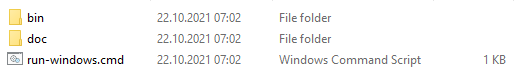
2. Extract the files and you will have a root folder looking like the figure below
3. Download the dp-ship demo case.
4. Extract the demo configuration
5. Run the startup script: run-windows.cmd
6. The application should open in your web browser at url http://localhost:8000.

Linux:

1. Download the cosim demo app.
2. Extract archive: tar -xzvf cosim-demo-app-vX.Y.Z.tar.gz
3. Download the dp-ship demo case.
4. Extract the demo configuration
5. Run startup script: run-linux
6. The application should open in your web browser at url http://localhost:8000.

back to top

Load a Configuration

Note: Each item below is highlighted in the figure below with its corresponding number.

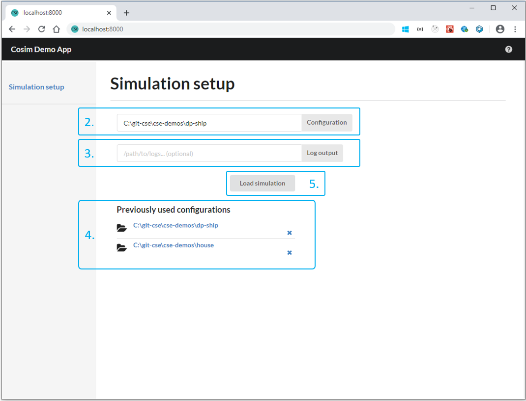
1. Switch to your web browser at url http://localhost:8000.
2. Enter the path to the dp-ship folder on your machine (for example: C:\cosim-demos\dp-ship)
3. Enter the path to a directory where you want the logs to be written. Leave it blank to disable file logging.
4. Previously used configurations are available below.
5. Click “Load simulation” to load the configuration.

A typical configuration folder will contain simulation models (FMUs) and configuration files. Connections between models and initialization values are configured through the files OspSystemStructure.xml or SystemStructure.ssd. If your configuration directory contains both (OspSystemStructure.xml and a SystemStructure.ssd), the .xml file will be prioritized. If you would like to load your simulation with the connections as defined on the SystemStructure.ssd file, include it in the path (Example: C:\cosim-demos\dp-ship\SystemStructure.ssd)

back to top

Observe models and variables

Note: Each item below is highlighted in the figure below with its corresponding number.

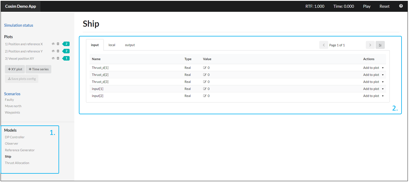
1. After loading the configuration, the simulation models are shown on the left hand side.
2. Browse the model variables by clicking the names. Their variables are organized in tabs based on causality.

back to top

Simulation control

Note: Each item below is highlighted in the figure below with its corresponding number.

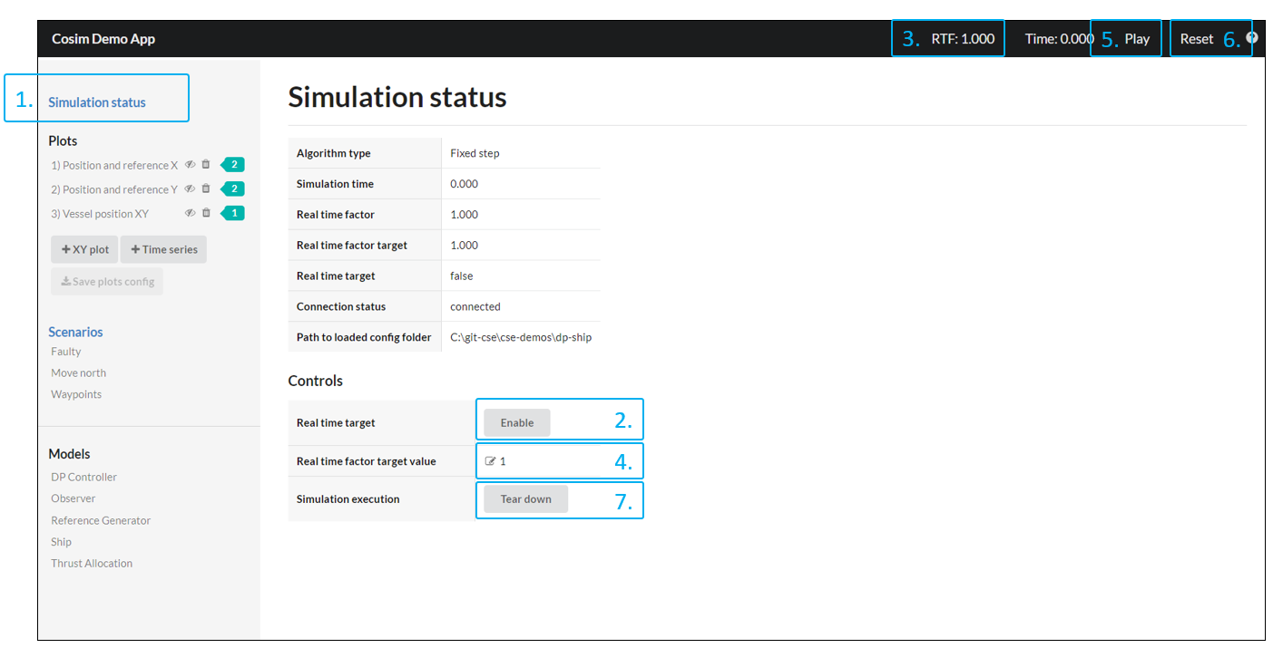
1. Click “Simulation status” to see details about the simulation and to access additional simulation control features.
2. By clicking “Enable” on the real time target, the simulation will run in real time. If real time target is disabled, the simulation will run in free mode (as fast as the hardware allows).
3. At the navigation bar, the RTF (Real Time Factor) indicates the current simulation speed related to real time. For instance, a RTF = 2 means that simulation runs at twice the speed of real time.
4. Real time factor target value can be altered to set a specific RTF.
5. At the navigation bar, click on “Play/Pause” to start or pause the simulation.
6. At the navigation bar, click on “Reset” to stop a simulation and initialize it again.
7. To close the current simulation and to load another configuration, click the “Tear down” button. Note that the current simulation needs to be paused in order to enable this button.

back to top

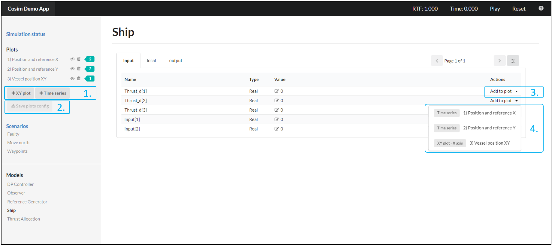
Plot variables

Note: Each item below is highlighted in the figures below with its corresponding number.

1. Click “+ XY plot” or “+ Time series” to create a new XY plot or a new time series plot, respectively. The plots are initially empty. Navigate to a simulation model and add variables to a plot.
2. Click “Save plot config” to save to file the current plot configuration. Next time the configuration is loaded the saved plots will be automatically loaded.
3. Any variable can be added to a plot by clicking “Add to plot” in the variable overview.
4. Select where to plot the variable from the list of available plots.
5. Click the plot name to see the chart.

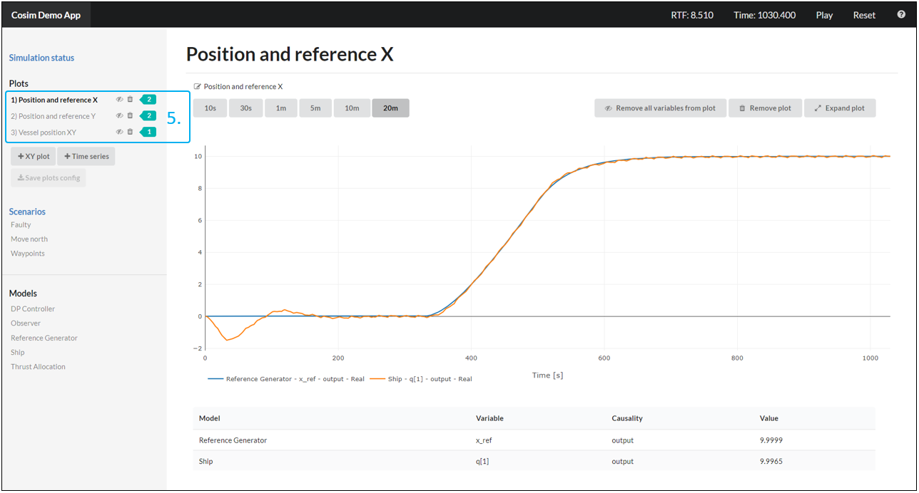
Configurable Plot

Two types of plot are supported by the cosim demo app: trend and scatter. The type trend (above defined as “time series”) shows the curve of a variable over time, while the type scatter (above defined as “XY plot”) shows the relation between two variables, of one versus the other.

In order to quickly setup the simulation environment, it is possible to store the plot configuration in a file. Start by creating a file named “PlotConfig.json” in the configuration folder. The file content is as defined in the example below. When the configuration is loaded the pre-defined plots will be automatically generated. In this configuration, simulator refers to the simulation models.

{
  "plots": [
    {
      "label": "label",
      "plotType": "trend",
      "variables": [
        {
          "simulator": "model name 1",
          "variable": "variable name 1"
        },
        {
          "simulator": "model name 2",
          "variable": "variable name 2"
        }
      ]
    },
    {
      "label": "Room temp XY",
      "plotType": "scatter",
      "variables": [
        {
          "simulator": "model name 1",
          "variable": "variable name 1"
        },
        {
          "simulator": "model name 2",
          "variable": "variable name 2"
        }
      ]
    }
  ]
}

back to top

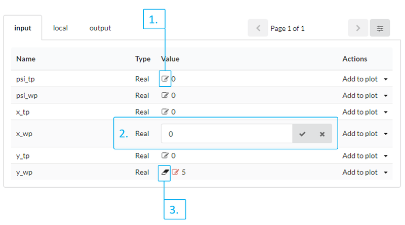
Override variable values

Note: Each item below is highlighted in the figure below with its corresponding number. It is possible to override any variable value.

1. Click the edit icon to the left of the variable.
2. Type in the value and click the check icon to confirm the new value.
3. Click the eraser symbol to remove the override.

back to top

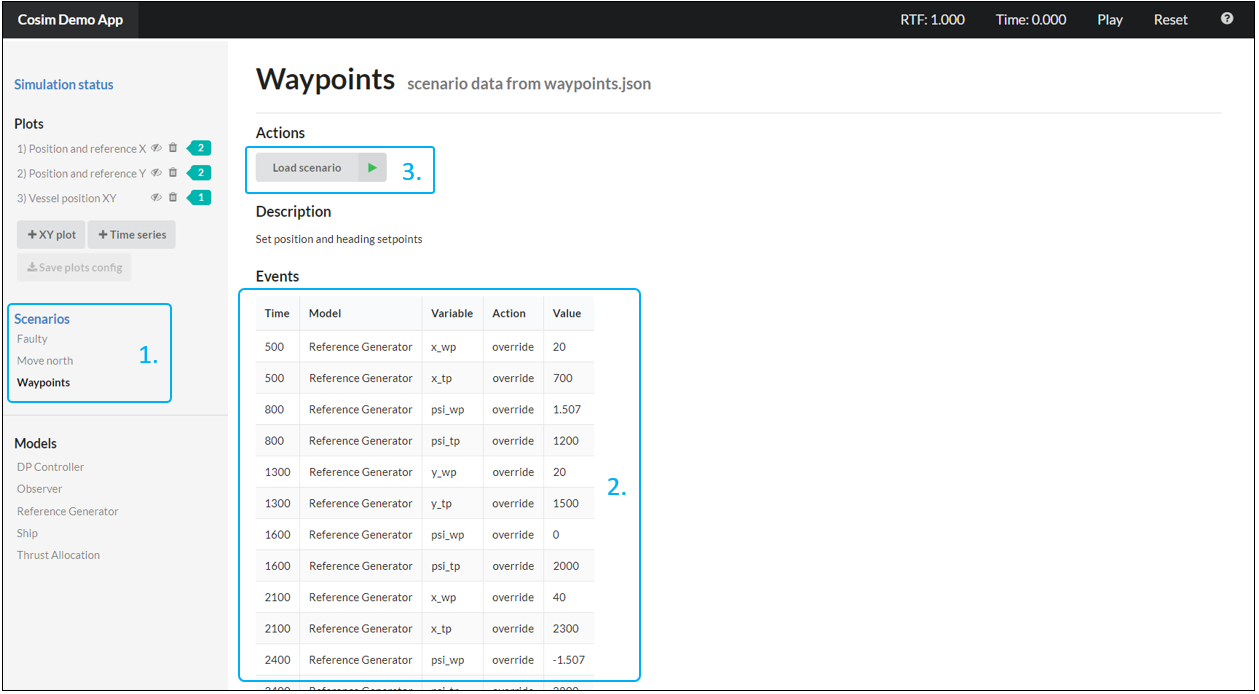
Run Scenarios

Note: Each item below is highlighted in the figure below with its corresponding number.

The scenario management allows to automatically change the value of variables at specified times. Each scenario is pre-defined on a file.

1. Scenario files placed in the ./scenarios subfolder within the configuration folder are automatically loaded and made visible in the “Scenarios” section. The dp-ship example comes with three scenario files for demonstration purposes. Click on each scenario to see its contents.
2. The “Events” section show a list containing when each variable value will be modified and to which value.
3. To execute a scenario click on “Load scenario”. The scenario will run and the variable values will be modified according the event list.

See more details on libcosim

back to top

Log simulation results

In order to log to file signal values from a simulation, an output directory must be specified in the “Log folder” field when loading a configuration. By default, all signals will be logged and persisted on every sample. There will be one file generated per simulator (simulation model). This can quickly lead to a large amount of data being stored, so it is recommended to specify which signals to log using the configurable log format as described here.

There is support for a basic configuration containing specific signals to be logged from any simulator model via an XML file. This file must be named “LogConfig.xml” (include the camel casing) and placed in the same folder as the configuration. See more details on libcosim.

back to top

Co-simulation configuration

The co-simulation configuration can be defined by either an “OspSystemStructure.xml” or by a “SystemStructure.ssd” file (using the SSP standard). These configuration files should be placed in the configuration folder. A few examples of what can be configured in such a file includes: connection between models, initial variable values or step size of a model.

The demo cases dp-ship, quarter-truck and house have in their configuration folder examples of both “OspSystemStructure.xml” and “SystemStructure.ssd” files.

The code below is an example of a “OspSystemStructure.xml” file:

<?xml version="1.0" encoding="UTF-8"?>
<OspSystemStructure xmlns="http://opensimulationplatform.com/MSMI/OSPSystemStructure"
                    version="0.1">
    <BaseStepSize>0.01</BaseStepSize>
    <Simulators>
        <Simulator name="ModelX" source="fmu1.fmu">
            <InitialValues>
                <InitialValue variable="input1">
                    <Real value="42"/>
                </InitialValue>
            </InitialValues>
        </Simulator>
        <Simulator name="ModelY" source="fmu2.fmu" stepSize="0.1"/>
        <Simulator name="ModelZ" source="fmu3.fmu" stepSize="0.05"/>
    </Simulators>


    <Connections>
        <VariableConnection>
            <Variable simulator="ModelX" name="model_output"/>
            <Variable simulator="ModelY" name="model_input"/>
        </VariableConnection>
    </Connections>
</OspSystemStructure>

If your configuration directory contains both (“OspSystemStructure.xml” and a “SystemStructure.ssd”), the .xml file will be prioritized. If you would like to load your simulation with the connections as defined on the “SystemStructure.ssd” file, include it in the path.

Note: The new OSP-IS connection types are not supported when using the SSP standard.

back to top

Distributed co-simulation using proxyfmu

Distributed simulation using proxyfmu allows you to run multiple instances of a model, run models that are not compatible with your operational system or to parallelize the workload onto multiple computation nodes. See more details on proxyfmu.

The demo case dp-ship has a specific configuration to be used with proxyfmu (see the file “OspSystemStructure.xml” or “SystemStructure.ssd” under the folder \proxyfmu). Note that the only difference when comparing to the regular configuration is related to the source of the FMU file.

Below is an example of how to specify proxyfmu sources for the “OspSystemStructure.xml”:

<Simulators>
	<Simulator name="FMU1" source="proxyfmu://localhost?file=path/to/fmu1.fmu"/>
	<Simulator name="FMU2" source="proxyfmu://localhost?file=file:///C:/path/to/fmu2.fmu"/>
	<Simulator name="FMU3" source="proxyfmu://127.0.0.1:9090?file=path/to/fmu3.fmu"/>
</Simulators>

Both relative and absolute file paths are supported, but absolute paths must begin with file:///. Also note that, when choosing localhost without specifying a port, new processes will automatically be spawned on the current system. If you need to run the model on a different PC, start proxyfmu_booter on the target PC and supply the IP and port to the configuration.

back to top